In special cases, if it is possible to write the exchange pattern of a Hamiltonian as a sum over complete graphs, we can use the spin quantum numbers of these graphs to recursively generate a complete list of eigenvalues without having to compute anything numerically.
Exchange Hamiltonian
Our goal is to investigate the physical properties of the Heisenberg model
$$
{\cal H}=\sum_{\langle ij\rangle}\sum_{\alpha\beta}
S_{i}^\alpha J_{ij}^{\alpha\beta}S_{j}^\beta.
$$
As an example, we will use S = 1/2 objects (spins) on the anisotropic
triangular lattice with an isotropic exchange in spin space, tiled by the
cluster displayed here.
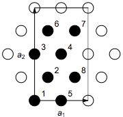
Eight-site cluster (black dots) tiling the infinite lattice with lattice
vectors a1 and a2. If periodic boundary conditions
are applied, the cluster forms a complete graph.
We define
$$
{\cal H}_{\cal L}^{\text{CG}}
:=
\sum_{i<j\in{\cal L}}
{\bf S}_{i}\cdot{\bf S}_{j}
=
\frac12\left[
\left(\sum_{i\in\cal L}{\bf S}_{i}\right)^{2}
-\sum_{i\in\cal L}{\bf S}_{i}^{2}
\right]
$$
as an exchange Hamiltonian for a collection of spins sitting on a list of
sites L. Because this Hamiltonian only depends on the square of the
total spin and the square of the spins on each site, we can replace these
operators by their respective list of quantum numbers and immediately get
the spectrum of the Hamiltonian.
Our Hamiltonian with nearest-neighbor exchange constants
J2 horizontally and J1 along the other two
directions on the eight-site tile shown above reads
$$
\begin{eqnarray*}{\cal H}_{8}
&=&
J_{1}\left[
{\cal H}_{\{1,2,3,4,5,6,7,8\}}^{\text{CG}}
-\left(
{\cal H}_{\{1,3,4,5\}}^{\text{CG}}+{\cal H}_{\{2,6,7,8\}}^{\text{CG}}
\right)
\right]
\nonumber\\&&{}
+2J_{2}\left[
{\cal H}_{\{1,5\}}^{\text{CG}}
+{\cal H}_{\{3,4\}}^{\text{CG}}
+{\cal H}_{\{2,8\}}^{\text{CG}}
+{\cal H}_{\{6,7\}}^{\text{CG}}
\right]\end{eqnarray*}
$$
with site labels as in the figure. Now we get the corresponding list of
eigenvalues by hierarchically constructing all possible multiple-spin
configurations starting with the basic two-spin singlets and triplets on
the pairs {1,5}, {3,4}, {2,8}, and {6,7}: From all pairs of two-spin
states, we can construct the four-spin states with total spin S = 0,1,2,
each possible pair of these four-spin states in turn can be combined to an
eight-spin state with total spin S = 0,1,2,3,4 and spin degeneracy (2
S+1). Because the total spin may be composed in several ways by the
spins of sub-clusters there exist additional degeneracies. In this way, we
can construct a total of 70 states for the eight-site cluster.
Eigenvalues
Here is the list:
$$
\small
\begin{array}{c|cccccc|c|c}
S_{1-8} & S_{1345} & S_{15} & S_{34} & S_{2678} & S_{28} & S_{67} &
\text{energy} &
\text{deg.} \\
\hline
0 & 0 & 0 & 0 & 0 & 0 & 0 & -6 J_2 & \;\;1* \\
0 & 0 & 0 & 0 & 0 & 1 & 1 & -2 J_2 & 2 \\
0 & 0 & 1 & 1 & 0 & 1 & 1 & 2 J_2 & 1 \\
0 & 1 & 0 & 1 & 1 & 0 & 1 & -2 \left(J_1+J_2\right) & 4 \\
0 & 1 & 0 & 1 & 1 & 1 & 1 & -2 J_1 & 4 \\
0 & 1 & 1 & 1 & 1 & 1 & 1 & 2 J_2-2 J_1 & 1 \\
0 & 2 & 1 & 1 & 2 & 1 & 1 & 2 J_2-6 J_1 &\; \;1* \\
1 & 0 & 0 & 0 & 1 & 0 & 1 & -4 J_2 & 4 \\
1 & 0 & 0 & 0 & 1 & 1 & 1 & -2 J_2 & 2 \\
1 & 0 & 1 & 1 & 1 & 0 & 1 & 0 & 4 \\
1 & 0 & 1 & 1 & 1 & 1 & 1 & 2 J_2 & 2 \\
1 & 1 & 0 & 1 & 1 & 0 & 1 & -J_1-2 J_2 & 4 \\
1 & 1 & 0 & 1 & 1 & 1 & 1 & -J_1 & 4 \\
1 & 1 & 1 & 1 & 1 & 1 & 1 & 2 J_2-J_1 & 1 \\
1 & 1 & 0 & 1 & 2 & 1 & 1 & -3 J_1 & 4 \\
1 & 1 & 1 & 1 & 2 & 1 & 1 & 2 J_2-3 J_1 & 2 \\
1 & 2 & 1 & 1 & 2 & 1 & 1 & 2 J_2-5 J_1 & 1 \\
2 & 0 & 0 & 0 & 2 & 1 & 1 & -2 J_2 & 2 \\
2 & 0 & 1 & 1 & 2 & 1 & 1 & 2 J_2 & 2 \\
2 & 1 & 0 & 1 & 1 & 0 & 1 & J_1-2 J_2 & 4 \\
2 & 1 & 0 & 1 & 1 & 1 & 1 & J_1 & 4 \\
2 & 1 & 1 & 1 & 1 & 1 & 1 & J_1+2 J_2 & 1 \\
2 & 1 & 0 & 1 & 2 & 1 & 1 & -J_1 & 4 \\
2 & 1 & 1 & 1 & 2 & 1 & 1 & 2 J_2-J_1 & 2 \\
2 & 2 & 1 & 1 & 2 & 1 & 1 & 2 J_2-3 J_1 & 1 \\
3 & 1 & 0 & 1 & 2 & 1 & 1 & 2 J_1 & 4 \\
3 & 1 & 1 & 1 & 2 & 1 & 1 & 2 \left(J_1+J_2\right) & 2 \\
3 & 2 & 1 & 1 & 2 & 1 & 1 & 2 J_2 & 1 \\
4 & 2 & 1 & 1 & 2 & 1 & 1 & 2 \left(2 J_1+J_2\right) & \;\; 1 *\\
\end{array}
$$
Those states marked with an asterisk have a classical analogon. Great, no
numerics involved!
Spectrum
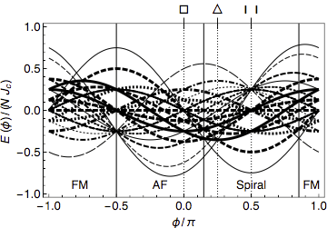
Spectrum of the anisotropic triangular Heisenberg model on an eight-site
complete graph. The thickness of the lines denotes the degeneracy, the
dashing distinguishes between different values of total spin Ω from
Ω = 0 (solid) to Ω = 4 (long-dashed). Parameter is the
anisotropy angle φ = tan-1(J2/J1).
Thermodynamics
With these eigenvalues we construct the partition function
$$
{\cal Z}=
\sum_{I}d_{I}\left(2S_{I}+1\right){\rm e}^{-\beta E_{I}}
$$
and its derivatives according to
$$
\begin{eqnarray*}\chi
&=&
% \frac{\beta J_{\text c}}N
\frac NV\mu_0\left(g\mu_\text B\right)^2\beta
\frac{1}{\cal Z}\sum_{I}
d_{I}(2S_{I}+1)\frac{S_{I}(S_{I}+1)}3
{\rm e}^{-\beta E_{I}},
\label{eqn:chieight}
\\
c_{V}
&=&
R\beta^{2}\left[
\frac{1}{\cal Z}\sum_{I}
d_{I}(2S_{I}+1)E_{I}^{2}{\rm e}^{-\beta E_{I}}
\right.
\nonumber\\
&\phantom{=}&
\hphantom{\frac{\beta^{2}}{N}}
\left.{}
-\left(
\frac{1}{\cal Z}\sum_{I}
d_{I}(2S_{I}+1)E_{I}{\rm e}^{-\beta E_{I}}
\right)^{2}
\right]
\end{eqnarray*}
$$
to get a sneak preview of what to expect in the thermodynamic limit. Here
SI is the total spin of state I (first column in the table),
EI its energy (next to last column) and dI is the
degeneracy of state I (last column).
Note to experimentalists: The susceptibility χ is dimensionless. For the dimension of the molar specific heat cV we use the universal gas constant R = NLkB where NL is the Loschmidt or Avogadro number.